Technologies that follow Wright’s Law get cheaper at a consistent rate, as the cumulative production of that technology increases.
The best way to explain what this means is to look at a concrete example.
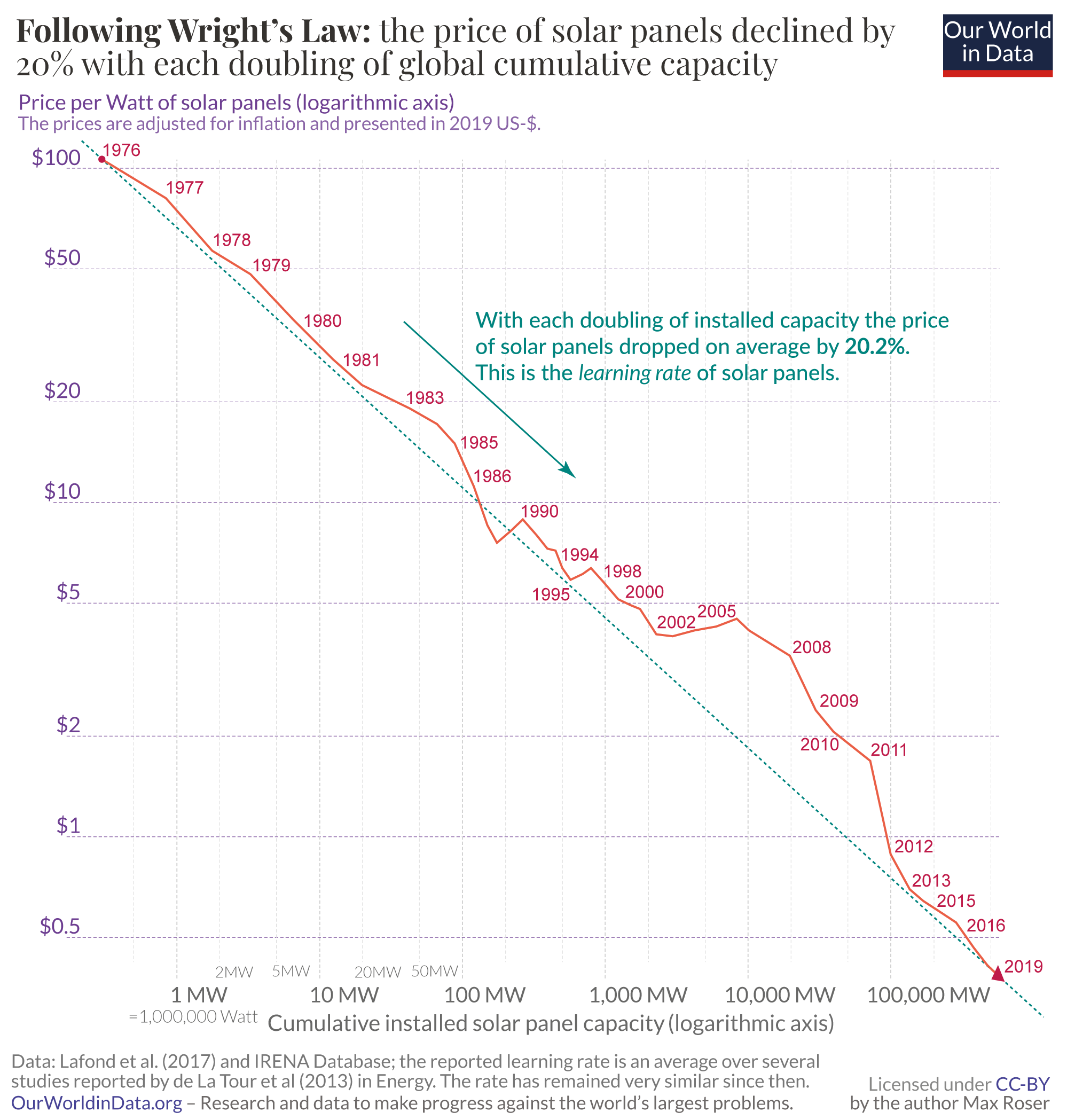
The time series in the chart shows the deployment of solar panels on the horizontal axis and the price of solar panels on the vertical axis. The orange line that describes the relationship between these two metrics over time is called the learning curve of that technology.
As the cumulative installed capacity increased, the price of solar declined exponentially. Solar technology is a prime example. For more than four decades, the price of solar panels declined by 20% with each doubling of global cumulative capacity.
The fact that both metrics changed exponentially can be nicely seen in this chart because both axes are logarithmic. On a logarithmic axis, a measure that declines exponentially follows a straight line.
That more production leads to falling prices is not surprising – such ‘economies of scale’ are found in the production of many goods. If you are already making one pizza, making a second one isn’t that much extra work.
What is exceptional about technologies that follow a learning curve is that this effect persists, and the rate at which the price declines stays roughly constant. This is what it means for a technology to follow Wright’s Law.
Solar power is not the only technology where we see trends of exponential change. The most famous case of exponential technological change is Moore’s Law – the observation of Intel’s co-founder Gordon Moore who noticed that the number of transistors on microprocessors doubled every two years.
We have another article on Moore’s Law on Our World in Data: What is Moore’s Law?
Integrated circuits are the fundamental technology of computers, and Moore’s Law has driven a range of changes in computer technology in recent decades – computers became rapidly cheaper, more energy efficient, and faster.
Moore’s Law, however, is not given in the same way that we just looked at for solar prices. Moore’s Law describes technological change as a function of time. In the example of solar technology we looked at price changes not as a function of time, but of experience – measured as the cumulative amount of solar panels that were ever installed.
This relationship that each doubling in experience leads to the same relative price decline was discovered earlier than Moore’s Law by aerospace engineer Theodore Paul Wright in 1936.1 It’s called Wright’s Law, after him.
Moore’s observation of the progress in computing technology can be seen as a special case of Wright’s Law.2
Solar panels are not the only technologies that follow this law. Look at our visualization of the price declines of 66 different technologies and the research referenced in the footnote3
The relative price decline associated with each doubling of cumulative experience is the learning rate of a technology.
The learning rate of solar panels is 20%. This means that with each doubling of the installed cumulative capacity, the price of solar panels declined by 20%.
In the footnote, you can find more information about the scientific literature on the learning rate in solar technology, and an example of how the learning rate is calculated.4
The high learning rate meant that the price of solar declined dramatically. As the chart above showed, the price declined from $106 to $0.38 per watt in these four decades. A decline of 99.6%.
That the price of technology declines when more of that technology is produced is a classic case of learning by doing. Increasing production gives the engineers the chance to learn how to improve the process.
This effect creates a virtuous cycle of increasing demand and falling prices. More of that technology gets deployed to satisfy increasing demand, leading to falling prices. At those lower prices, the technology becomes cost-effective in new applications, which in turn means that demand increases. In this positive feedback loop, these technologies power themselves forward to lower and lower prices.
The specifics, of course, differ between the different technologies. For more information on what is behind the price reduction of solar panels, see the footnote.5
How do we know that increasing experience is causing lower prices? After all, it could be the other way around: production only increases after costs have fallen.
In most settings, this is difficult to disentangle empirically, but researchers François Lafond, Diana Greenwald, and Doyne Farmer found an instance where this question can be answered. In their paper “Can Stimulating Demand Drive Costs Down?”, they study the price changes at a time when reverse causality can be ruled out: the demand for military technology in the Second World War. In that case it is clear that demand was driven by the circumstances of the war, and not by lower prices.6
They found that as demand for weapons grew, production experience increased sharply, and prices declined. When the war was over and demand shrank, the price decline reverted back to a slower rate. It was the cumulative experience that drove a decline in prices, not the other way around.
If you want to know what the future looks like, one of the most useful questions to ask is which technologies follow a learning curve.
Most technologies do not follow Wright’s Law – the prices of bicycles, fridges, or coal power plants do not decline exponentially as we produce more of them. But those which do follow Wright’s Law – like computers, solar panels, and batteries – are the ones to look out for. In their infancy, they might only be found in very niche applications, but a few decades later they are everywhere.
This means that if you are unaware that a technology follows Wright’s Law, you can get your predictions very wrong. At the dawn of the computer age in 1943, IBM president Thomas Watson famously said, “I think there is a world market for maybe five computers.”7 At the price point of computers at the time, that was perhaps perfectly true, but what he didn’t foresee was how rapidly the price of computers would come down. From their initial niche computers expanded to more and more applications, and the virtuous cycle meant that the price of computers declined continuously. The exponential progress of computer technology expanded their use from a tiny niche to the defining technology of our time.
Solar panels are on the same trajectory as we’ve seen before. At the price of solar panels in the 1950s, it would have sounded quite reasonable to say, “I think there is a world market for maybe five solar panels.” But as a prediction for the future, this statement too, would have been ridiculously wrong.
To get our expectations about the future right, we are well-advised to take the exponential change of Wright’s Law seriously. Doyne Farmer, François Lafond, Penny Mealy, Rupert Way, Cameron Hepburn, and others have done important pioneering work in this field. A central paper of their work is Farmer’s and Lafond’s “How predictable is technological progress?”.8 The focus of this research paper is the price of solar, so that we avoid repeating Watson’s mistake with renewable energy. They lay out in detail what I discussed here: how solar panels decline in price, how demand drives this change, and how we can learn about the future by relying on these insights.
To get our expectations for the future right, we need to pay particular attention to the technologies that follow learning curves. Initially, we might only find them in a few high-tech applications, but the future belongs to them.